What data mining is, how this course is run, and why you should tread with caution — this year with an information-access focus.
A. Anand (head lecturer) · with J. Urbano & N. Tömen · lecture 1 study deck
Part I
There are no correct answers — only correct design decisions
Data mining is a craft of choices under messy data. The next two stories — a cholera map in 1854
and an ancient library — are really design decisions about what structure to look for.
Question
London, 1854: hundreds are dying of cholera and no one knows why. All you have is a list of the addresses of the dead. How would you find the cause?
No germ theory yet, no microscope data — just locations on a map.
Think — then → for the answer.
London, 1854
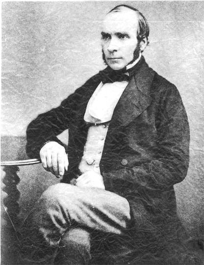
The first data miner — John Snow
The problem
A cholera outbreak tore through Soho —
~600 people dead in days.
The accepted theory was “bad air” (miasma). Nobody knew the real cause.
Snow, a physician, suspected the water — but had no proof.
All he had was a list of addresses of the dead. How do you find a cause in that?
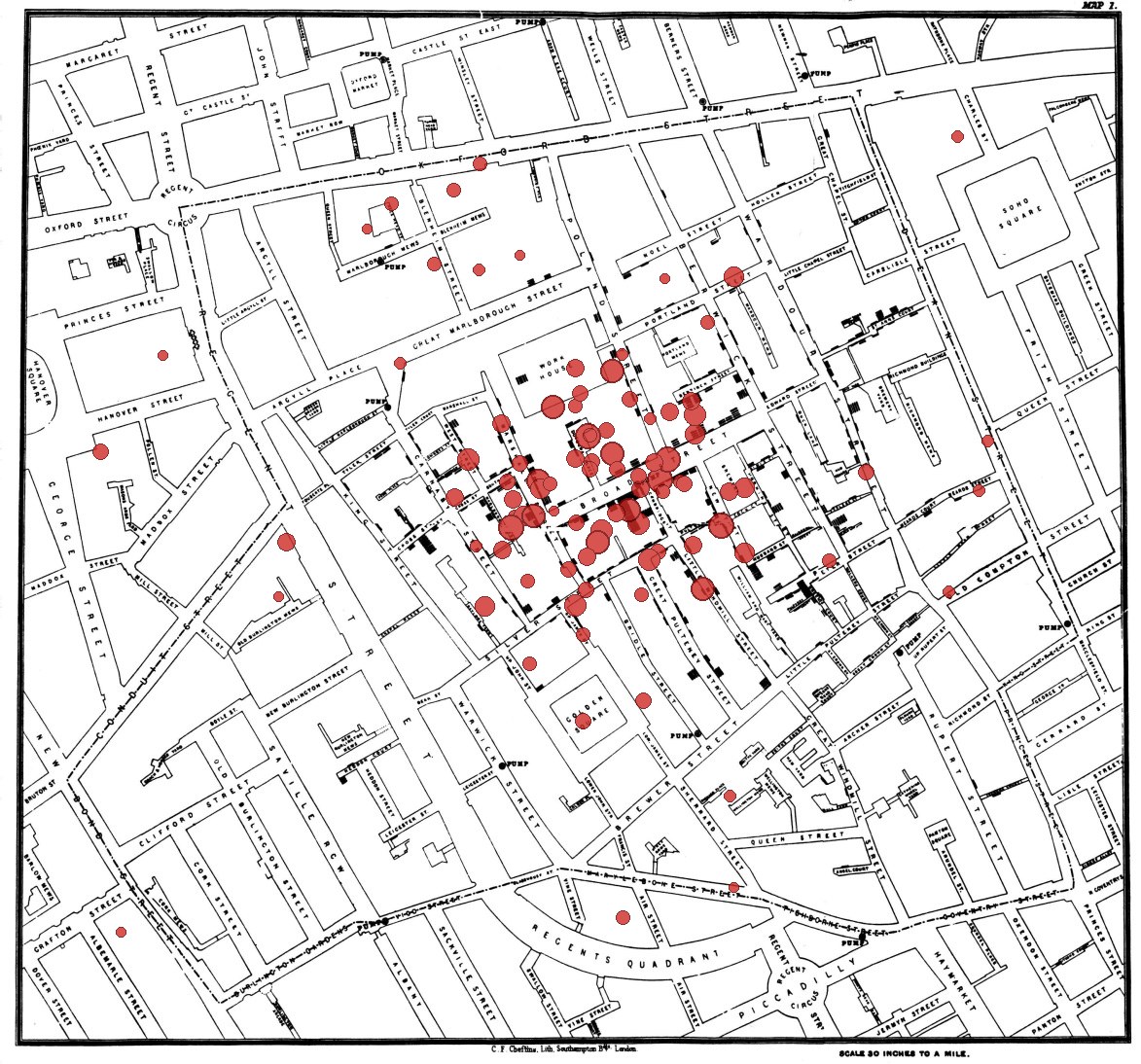
He plotted every death on a map
Each red dot is a cholera death. Snow marked them street by street — and a
dense cluster began to emerge in the middle of Soho, while whole blocks nearby stayed clear.
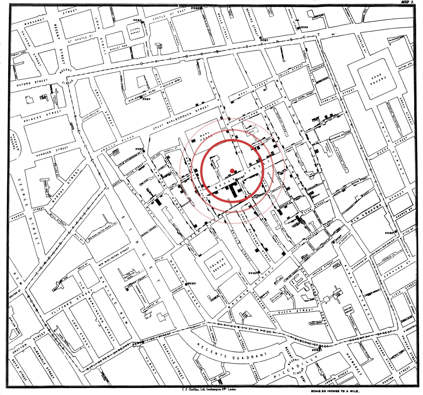
One pump explained it all
The deaths ringed one water pump on Broad Street. Snow had its handle removed — and the
outbreak stopped. The design decision — plot deaths in space, not in a table — made the cause visible.
Alexandria, 3rd century BC
Another origin story — the first retrieval system
~500,000 scrollsan unusable pile
→
The Pinakes cataloguegenre · author · title
→
Any scroll, foundinformation retrieval
How the Pinakes organized it
Callimachus catalogued the Library of Alexandria — the Pinakes (“tables”), arguably the first
information-retrieval system.
It split ~half a million scrolls into about ten genres (rhetoric, law, epic, history, medicine…);
within each, authors were listed alphabetically, each with a short biography; and every work was recorded
by its title, opening line, and line count. Any scroll was now locatable — the first real index.
The course definition
What data mining is — in this course
Working definition
Data mining is the craft of deciding what
structure to look for in large, messy, unlabelled data — and finding it at scale.
Deciding what to look for — the design decision, as in Snow’s map and the Pinakes.
Large, messy, unlabelled · at scale — the part of the problem this course focuses on.
A sharper slice of the broader textbook definition (“extract useful information from data”): we
emphasise scale and no labels.
blogs.sas.com
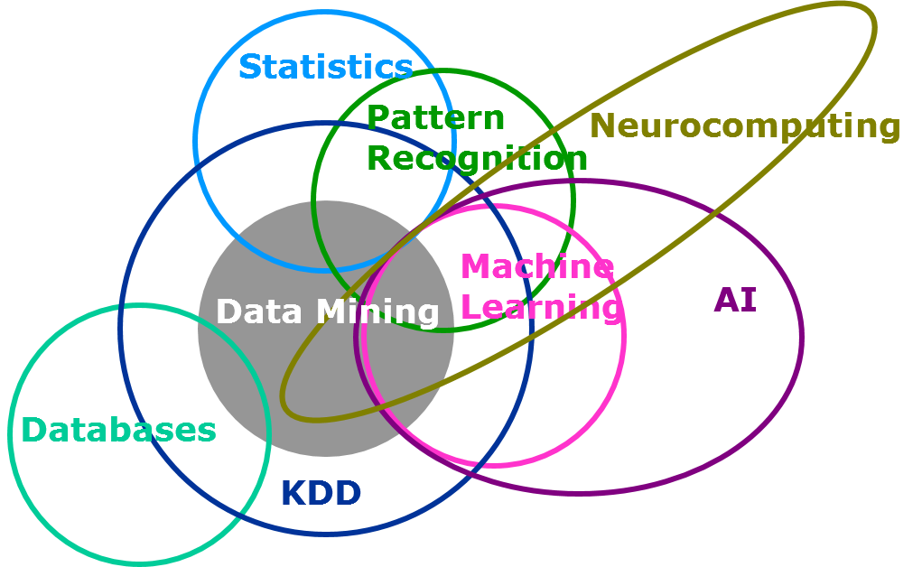
Data mining sits at an intersection
It borrows from statistics, databases, machine learning, pattern recognition and AI
— the overlap at the heart of Knowledge Discovery in Databases (KDD).
The broader textbook view
The textbook definition
Classic definition
The primary goal of data mining is to extract useful
information from a large volume of data and transform it into an
understandable structure for further use.
“…searching and analyzing a large batch of raw data to identify patterns and extract useful information.”
“…the development of models for data in order to extract information from it.”
“…analyzing data from different perspectives and summarizing it into useful information.”
Data mining vs. machine learning vs. data management
Raw datadata management
→
Explore & form the questiondata mining
→
Fit a modelmachine learning
→
Interpret · insightdata mining
Data management — store & serve the dataData mining — exploration & question-formulation (and making sense of the result)Machine learning — fitting the model
One shared pipeline — data mining frames the question, machine learning fits the model.
Recap
Where data mining lives
The division of labour
Machine learning owns the model-fitting stage — which algorithm, how to train it, the resulting model.
Data mining owns the exploration and question-formulation stage — deciding what to look for and what
“similar”, “structure”, or “relevant” should mean — and then making sense of the result. Often the data is
unlabelled, so the learning here is unsupervised.
A healthcare example
Mining first, then predicting
Data mining phase
Analyse a large database of patient records — symptoms, diagnostics, treatments, outcomes —
with clustering, association rules, pattern discovery to uncover patterns
(e.g. fever + cough + shortness of breath → a specific respiratory illness).
Machine learning phase
Use those discovered patterns to train a model. A new patient’s symptoms →
the model predicts likely diagnoses and suggests treatments from historical success rates.
Data mining finds the structure; machine learning predicts with it.
Cyber security · malware families
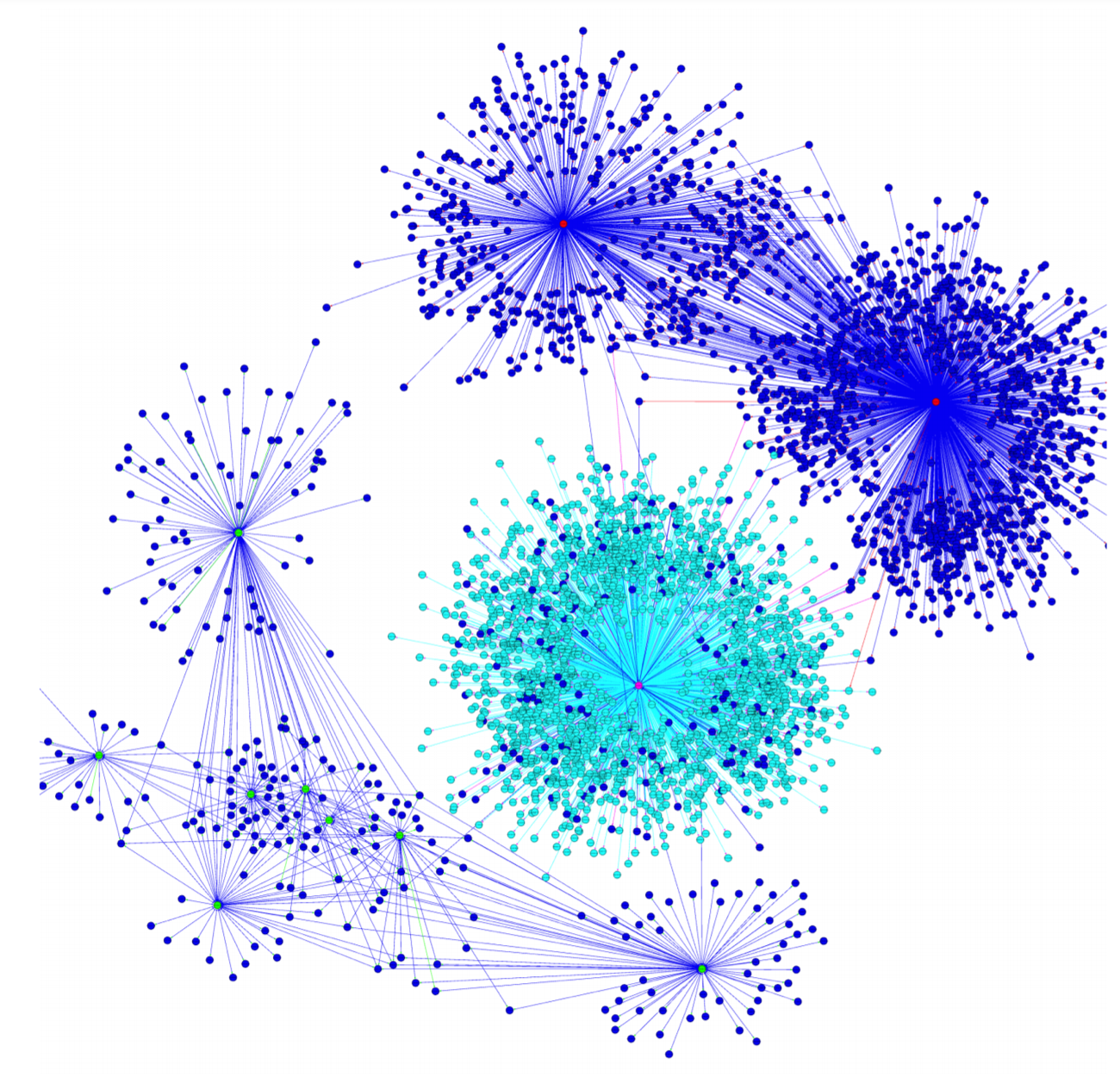
A real example: network / graph data
Connections between hosts form a huge graph. Clustering it reveals behavioural
profiles of malware families — no labels needed (Nadeem et al., 2020).
Making the result insightful
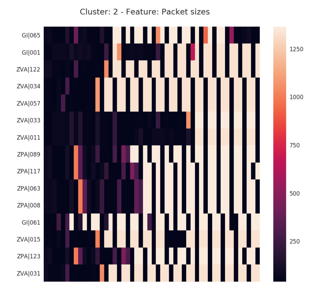
Visualise groups with heatmaps
Row = connection · column = time · cell colour = bytes transferred.
A cluster becomes a readable behavioural signature.
The whole loop
These are all data-mining skills
The data-mining loop
Take the data as is, but select features using domain knowledge →
cluster with clustering methods → make the gained knowledge insightful (e.g. heatmaps).
Feature choice, the right algorithm, and a human-readable result — that end-to-end judgement is the craft.
The three V’s
Why is data mining hard?
Volume
Too big to fit / scan naively
Need scalable algorithms
Velocity
Data arrives fast / streams
Need approximate yet accurate estimates
Variety
Many types & distributions
Must adapt methods to each
These three pressures are exactly why we need hashing, indexing, embeddings and dimensionality reduction.
Part II
The course & logistics
The team, what’s new this year, and how everything runs — goals, schedule, labs, grading, prerequisites.
Who teaches this course
Three instructors, three verticals
Avishek Anand · head lecturer
Assoc. prof., Web Information Systems
IR, NLP, Explainable AI
Teaches: distances, embeddings, graphs — text & graph mining
Julián Urbano
Asst. prof., Computer Science (TU Delft)
Music IR, retrieval evaluation, significance testing
The course is reoriented around information access — how we find, rank, and evaluate
the right information inside massive data, not just describe it.
Content swap vs. last year: out go anomaly detection and sketching; in come
retrieval, ranking, and evaluation.
One lab assignment this year — down from two.
No Kaggle competition this year.
New reading: Introduction to Information Retrieval (Manning, Raghavan & Schütze) for selected chapters.
What you should walk away with
Course goals — three strands in every lecture
The promise
Each lecture runs three strands at once — the concepts,
the algorithms, and the
skills to apply them.
Concepts
The ideas & theory
Which concept fits which data type
Algorithms
Implement them from scratch
Strengths, weaknesses, and when to use them
Skills
Pick the right method for a problem
Make it work on real, messy data
The skills strand lives mainly in the lab project — where you apply concepts & algorithms end-to-end.
The spine of the whole course
Three verticals: Distances · Matrices · Retrieval
Distances · Avishek
“When are two things similar — and who decides?”
Similarity & metrics, DTW
Text & graph embeddings
Clustering · Hashing · MinHash / LSH
Matrices · Nergis
“What hidden structure explains the data?”
Representation & operations
Factorization & decompositions
Dimensionality reduction (PCA)
Retrieval · Julian
“How do I find the right thing fast — and how do I know I did?”
Indexing & the inverted index
Ranking · Evaluation
Near-duplicate / similar-item search
This year’s shift: counting folds into Distances, and Retrieval becomes its own vertical —
the information-access focus. Every topic hangs off one of these three.
In the room we do case studies — how do you actually apply what you learned to a real problem?
Complete schedule lives on Brightspace.
Where the content comes from
Course material
On Brightspace (required)
Lecture slides (after each class), lab exercises (start of each week), and reading materials
— selected book chapters and papers.
Free via the TU Delft digital library: Mining of Massive Datasets · Data Mining.
New this year — Introduction to Information Retrieval (Manning, Raghavan & Schütze)
for the retrieval / ranking / evaluation chapters.
Free online: nlp.stanford.edu/IR-book
Only the selected chapters uploaded to Brightspace are examinable.
Mandatory · in groups
Lab sessions
One lab assignment this year, in groups — Tuesday mornings (08:45), help and feedback on the spot.
Two parts: algorithm implementation (Distances / Matrices / Retrieval) and a pipeline
(transform → analyse → visualise), built from scratch — no scikit-learn. No Kaggle this year.
Each group submits one solution, then peer-reviews 2 other groups’ assignments on Peer.
Register your group on Brightspace this week — little flexibility: groups are exported to Peer soon so grading stays on time.
Missed or failed? An “Assignment repair” resit is due 2 weeks after the original deadline.
Help: Queue, Mattermost, Answers EWI (tag CSE2525), Weblab, Peer. Please do not use e-mail.
Lab 3 × 10% · Exam 70%
Assessment & grading
How the grade is made up
Lab = 30%, split into three 10% parts — algorithm implementation (auto-graded), the pipeline
(peer-reviewed), and your peer reviews. Exam = 70%. No Kaggle this year.
To pass (TER Art 29, sub 4): each graded element must be > 5.0,
and the final computed grade (exam + lab) must be > 5.8. Check the TER.
The assessment
Final exam
Final exam = 70%, on WebLab (Osiris + WebLab registration). Open and multiple-choice questions.
No programming questions this year · closed book, calculator allowed · one resit.
A practice exam will be available — one only this year, due to staff & topic changes.
No partial transfer from previous years. mytimetable.tudelft.nl is authoritative for dates.
What we assume you already know
Expected prior knowledge
Discrete maths — sets, intersections, unions.
Linear algebra — matrix multiplication, projections, eigenanalysis.
Probability & statistics — Gaussians, correlation, covariance.
Data structures — hash tables and indexes. Programming — Python.
Machine learning — logistic regression, random forest, SVM, …
Based on CSE1100/1305/1200/1205/1210 and CSE2510/2520. Not enforced —
you are responsible for your own study success.
Recap of Part I
Logistics in one slide
Key points
One mandatory lab — 3 × 10% (algorithm + pipeline + peer reviews); exam 70%.
Pass needs > 5.0 on each element and > 5.8 overall (TER Art 29.4).
Register your lab group this week.
This year’s focus: information access — retrieval, ranking and evaluation replace anomaly
detection and sketching. Feedback only: dm-cs-ewi@tudelft.nl.
Part III
A word of caution
Don’t fool yourself. The rest of this lecture is cautionary tales about results that look great and are wrong.
WWII · Abraham Wald
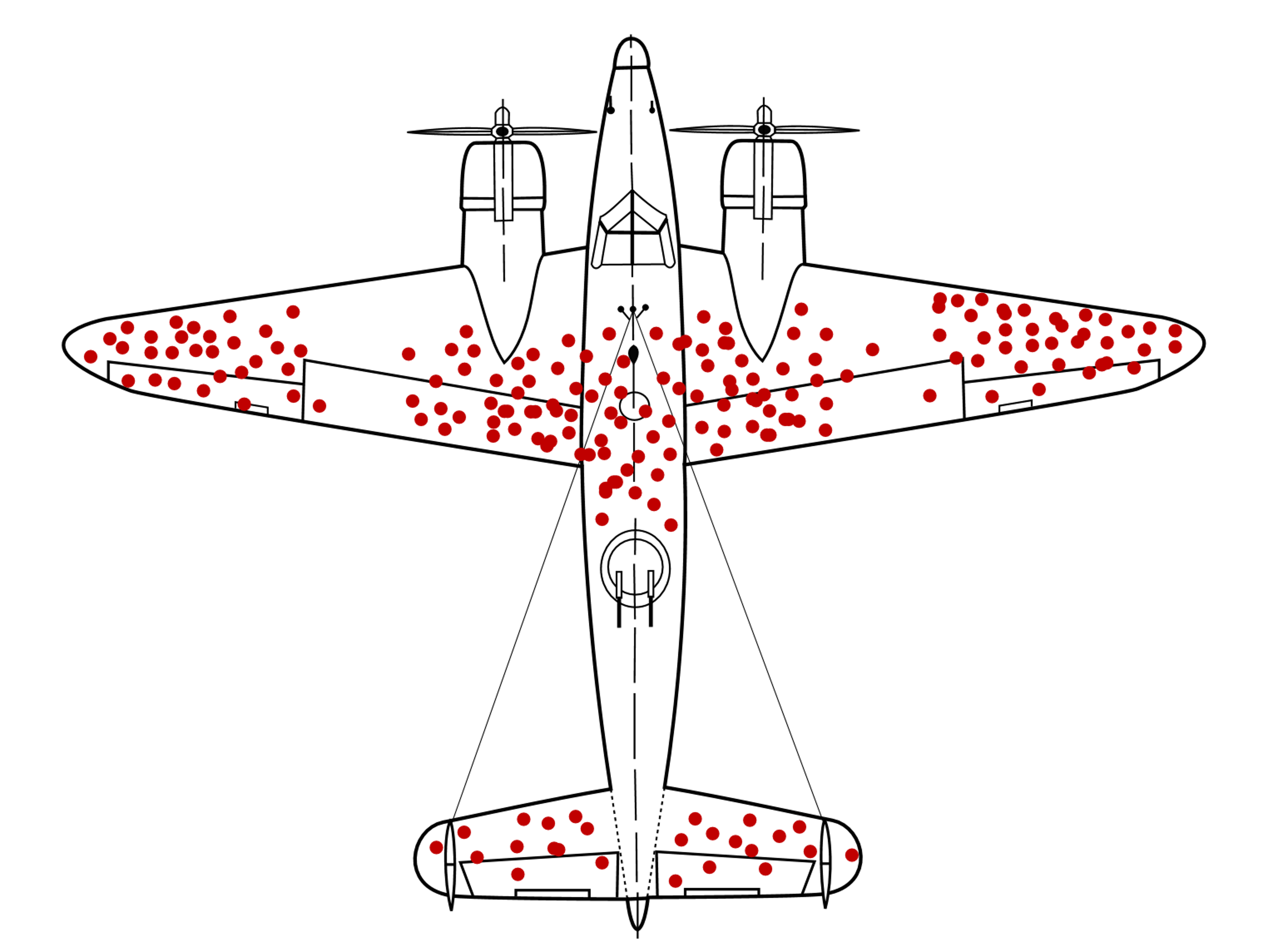
Survivorship bias
Red dots = damage on planes that returned. Where should you add armour?
Not where the dots are — where they aren’t (engines, cockpit): planes hit there never came back.
Your data is only the survivors.
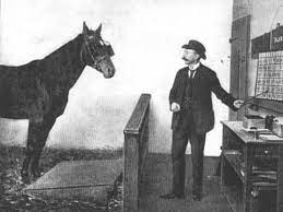
The horse that could “count”
The Clever Hans effect
Hans seemed to do arithmetic — but was really reading his trainer’s unconscious cues.
Models do this too: right answer, wrong reason.
Too good to be true
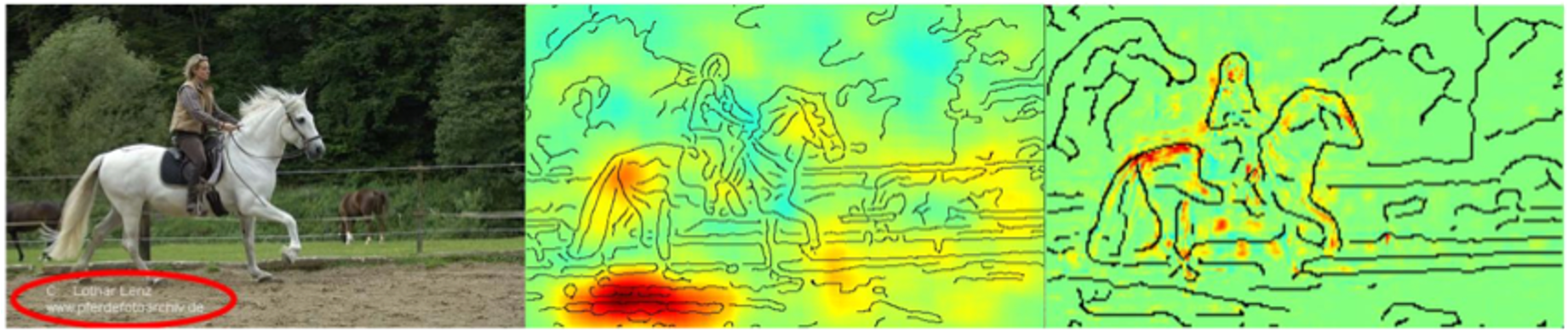
Shortcuts in learning — Wikipedia citations
The task
Automatically predict which Wikipedia sentences need a citation.
A neural network scored 100% on the test set — while humans agreed only <55% of the time.
What should you ask?
100% accuracy on a task humans find genuinely hard is too good to be true — a red flag, not a trophy.
The catch: sentences needing a citation already carried the marker “[ ]”. The model learned
“if the bracket is there, predict citation-needed” — a shortcut, not understanding.
The canonical ML parable
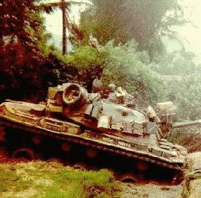
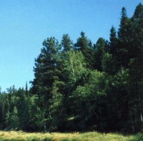
Shortcut learning — the “Russian tanks”
100% accurate in training, worse than random on new data. The network had learned:
“if the sky is blue, no tank; otherwise, tank.”It classified the weather, not the tanks.
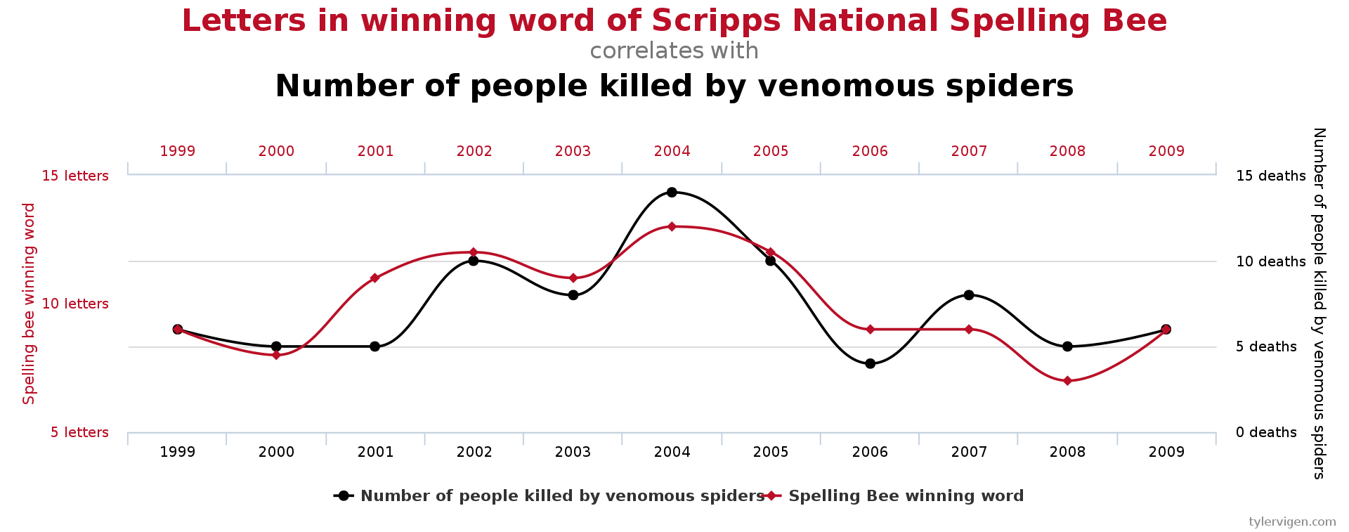
Test enough hypotheses and some will “correlate” by pure chance.
The multiple-comparisons problem is the cause of many data-mining errors — significance you went fishing for isn’t significance.
Lecture 1 · wrap-up
Summary
Take away
Data mining = extract useful information from a large volume of data and turn it into an
understandable structure. It focuses on the input and output ends of the ML pipeline, often unsupervised.
Organised around three verticals — Distances · Matrices · Retrieval. Grading: labs 30%,
exam 70%.
It’s called the skill of the 21st century — but tread with caution. Survivorship bias, Clever Hans,
shortcut learning and multiple comparisons are waiting to fool you.