Choosing a distance is choosing which patterns an algorithm can see — worked through two case studies.
A. Anand · study deck
In this lecture
Distances & similarity — the roadmap
Almost every mining task — classify, cluster, flag outliers, search — reduces to one question:
what is close to what? This lecture is about the decision hiding behind it: the distance.
Design decisions: task → representation → distance → decision rule — and why choosing them is choosing the model.
Metrics: the four axioms, why metric structure helps (pruning), and the pitfalls — cosine and squared-Euclidean are not true metrics.
Representations: vector, set, sequence, graph — each with its own distance (even text can be a dense vector).
Two real-world case studies: product recommendation (which differences matter) and near-duplicate detection (which to ignore).
Part I
Why distance underlies data mining
Before any formula: what does a distance actually let us do?
The one idea to hold onto
Choosing a distance is choosing what’s similar
Every task today — classify, cluster, flag outliers, search — reduces to one question:
what is close to what? Change the distance and the answer changes, though no data point moved.
The query ★ is a running shoe; the candidates are a dress shoe and another running shoe. Its nearest neighbour flips: dress by price, running by purpose.
“Similar” has no default meaning — it depends what you measure:
Similar in price? — a running shoe lands next to a dress shoe.
Similar in purpose? — it lands next to other running shoes.
Similar in description text? — grouped by words, not by use.
Similar in who buys it? — you get complements, not substitutes.
Same two candidates, same query — the nearest neighbour flips with the distance. The task decides which sense you want; the distance is how you encode it.
Distance is a shared building block
One dataset — four questions
Mining task
The question, expressed through distance
Classification
Which labelled examples are closest to this new object?
Clustering
Which objects are close enough to form groups?
Anomaly detection
Which objects are far from the usual observations?
Similarity search
Which existing objects are closest to this query?
Your turn · 2 min with your neighbour
Design decision: the “more like this” button
Scenario
A music app wants a “more like this” button on every song. You decide what powers it.
Which of today’s four questions is this — classification, clustering, anomaly, or similarity search?
What should “similar” mean here — same genre, same tempo & mood, or the same listeners?
Each answer is a different representation. Which one can you actually compute from the data you have?
There’s no correct answer — only a design decision you can defend. We’ll compare a few.
Part II
Task → representation → distance
The choice of distance is the model — so make the choice deliberately.
From intuition to vocabulary
Features, and what we mean by a “model”
Feature
A measurable property of an object — its price, its category, the words in its description, who buys it.
Representation
The features you choose to describe an object — its encoding. We formalise this as a representation space next.
Model (here)
Representation + distance + decision rule. Choosing the features and the distance is choosing the model.
Different features give different neighbours — so the modelling decision begins by choosing features, which we assemble into a representation space next.
Before the distance comes the encoding
What is a representation space?
Definition
A representation encodes each object as an element of a chosen space ℛ — a vector, a set, a sequence,
a node in a graph. Every later step sees only what ℛ records, so two objects identical in ℛ are
indistinguishable to the distance. Choosing ℛ is the first modelling decision.
Vector · ℝⁿ
object → a point of numeric features
Euclidean · cosine
Set
object → a set of elements (words, shingles)
Jaccard
Sequence
object → an ordered string of symbols
edit · Hamming
Graph / tree
object → a node in a graph
shortest path
Your turn · match the data to the space
What is a representation space?
Question
You’ve met four spaces — vector, set, sequence, graph. For each, name a kind of data that fits it best.
Then the twist: could the same object live in more than one?
Vector · ℝⁿ
numeric data — sensor readings, pixels
Set
the words in a document
Sequence
a time series · text characters
Graph / tree
a social network · the web
The catch: the same text is a set of words, a sequence of characters — or a dense vector (embeddings, next lecture). The representation is a choice, not a given.
Vector space · the straight-line distance
Euclidean distance
The distance is the hypotenuse: √(3² + 4²) = 5.
d(x, y) = √( Σi (xi − yi)² )
Worked example
x = (1, 2), y = (4, 6).
d = √((4 − 1)² + (6 − 2)²) = √(9 + 16) = √25 = 5.
Cosine is its sibling for text — it compares direction, not magnitude. We’ll meet both again: where they’re used, and whether they’re metrics.
Set · the overlap of two sets
Jaccard distance
∩ = {c, d} = 2 · ∪ = 5 → J = 0.4, d = 0.6.
J(A, B) = |A ∩ B| / |A ∪ B| dJ= 1 − J(A, B)
Worked example
A = {a, b, c, d}, B = {c, d, e}.
A ∩ B = {c, d} → 2, A ∪ B = {a, b, c, d, e} → 5. J = 2/5 = 0.4, dJ = 0.6.
Natural for documents seen as sets of words or shingles. We’ll meet it again — in near-duplicate detection — and ask whether it’s a metric.
Sequence · how many edits apart
Edit (Levenshtein) distance
book → back: two substitutions → 2 edits.
d(x, y) = fewest insertions, deletions & substitutions turning x into y
Worked examplebook → back: b·b ✓, o → a, o → c, k·k ✓ → 2 substitutions.
Equal length, substitutions only → this coincides with the Hamming distance. Insertions & deletions let it compare different lengths: book → books = 1.
We’ll meet Hamming again in Part III — where we prove it is a metric — and in the video case study.
Graph · the fewest steps between nodes
Shortest-path (geodesic) distance
Direct A–C = 5, but A–B–C = 1 + 1 = 2 wins.
d(u, v) = min over paths u → v of Σ weight(edges)
Worked example
Edges: A–B = 1, B–C = 1, and a direct A–C = 5.
Paths A → C: direct = 5, via B = 1 + 1 = 2. So d(A, C) = 2 — the shortest path wins.
Unweighted graphs → just count edges. We’ll work this out in full in Part III, and again in graph mining.
Four decisions, in order
Task → representation → distance → decision
Choice
What it determines
Task
What “similar” should mean
Representation
What information is available for comparison
Distance
Which differences matter, and how much
Decision rule
What we do with the resulting distances (e.g. top-k)
And you don’t always need a vector first — trees, strings and sets have distances directly.
Your turn · walk the sequence
Design decision: spot duplicate news articles
Scenario
A news aggregator scrapes the same story from dozens of sites, each with small edits. You must group the duplicates — fill in the four decisions.
Decision
Your call for this task
Task
What should “similar” mean — near-identical wording?
Representation
A set of words/k-grams? a vector of the text? or the whole string (a sequence)?
Distance
Each representation brings its own: Jaccard (set) · cosine (vector) · edit distance (string).
Decision rule
Group two articles when the distance is below which threshold?
Notice the dependency: the representation you pick decides which distances are even available to you.
Part III
Metrics as useful guarantees
What properties make a distance predictable — and fast?
Definition
When is a distance a metric?
Metric space
A function d : X × X → ℝ is a metric on a set X if, for every x, y, z ∈ X, it satisfies the four
axioms below. The pair (X, d) is then called a metric space.
Axiom
Formal statement
Non-negativity
d(x, y) ≥ 0
Identity of indiscernibles
d(x, y) = 0 ⟺ x = y
Symmetry
d(x, y) = d(y, x)
Triangle inequality
d(x, z) ≤ d(x, y) + d(y, z)
Triangle inequality: the detour x→y→z is never shorter than going direct.
Why these axioms are worth demanding
The axioms are guarantees an algorithm can exploit
c is ≥ 8 from q, but we only want neighbours within 3 — so c is skipped, unmeasured.
Identity and symmetry make “the nearest object” well-defined and independent of comparison order.
The triangle inequality lets known distances bound unknown ones, so candidates can be ruled out without measuring them.
Pruning with the triangle inequalityq is at distance 10 from a reference r; a candidate c is at distance
2 from r. The triangle inequality forces a lower bound:
d(q, c) ≥ |10 − 2| = 8. Since 8 > 3, c cannot be within 3 of q —
discard it without ever computing d(q, c).
This powers metric indexes — ball trees, VP-trees — that avoid the full O(n²) comparisons.
Exercise · check the axioms
Is the Hamming distance a metric?
Candidate distance
For strings x, y of equal length n, let dH(x, y) be the number of positions at which they differ.
Work through each of the four axioms for dH — does it hold?
For the ones that hold, give the reason; for any that fails, a counterexample.
Decide for yourself: is dH a metric? We’ll work it through together on the next slide.
At one position: xᵢ=yᵢ but yᵢ≠zᵢ, so xᵢ≠zᵢ — at least one pair always differs.
Proof — verify each axiom
Non-negativity.dH is a count of positions, hence dH(x, y) ≥ 0.
Identity.dH(x, y) = 0 ⟺ no position differs ⟺ x = y.
Symmetry. “position i differs” is the same statement for (x, y) and (y, x), so dH(x, y) = dH(y, x).
Triangle inequality. Fix a position i. If xi ≠ zi, then xi and zi
cannot both equal yi, so xi ≠ yioryi ≠ zi. Hence at each position
[xi≠zi] ≤ [xi≠yi] + [yi≠zi]. Summing over all n positions gives
dH(x, z) ≤ dH(x, y) + dH(y, z). ∎
At each index the distance is at most 1 (0 if equal, 1 if different), and [xi≠zi] ≤ [xi≠yi] + [yi≠zi] holds index by index — so summing over all indices, the total d(x,z) ≤ d(x,y) + d(y,z).
Exercise · find the broken axiom
Is squared Euclidean distance a metric?
Candidate distance
On ℝⁿ, define dsq(x, y) = ‖x − y‖² = Σi (xi − yi)² — the squared Euclidean
distance (the quantity k-means minimises).
Three of the four axioms clearly hold. Which one can fail?
Try to build a counterexample that breaks it.
Work on it first — the next slide gives a hint, and the one after that the full solution.
Direct (4) > detour sum (2) — so d(x,z) ≤ d(x,y)+d(y,z) is broken.
Counterexample on the real line
Take x = 0, y = 1, z = 2. Then
dsq(x, z) = (2 − 0)² = 4, while
dsq(x, y) + dsq(y, z) = 1² + 1² = 2.
So 4 > 2 — the triangle inequality is violated.
Takeaway
Non-negativity, identity and symmetry all hold, yet dsq is not a metric. Squaring breaks the triangle
inequality — which is why the Euclidean distance (its square root) is used wherever metric structure is required.
A metric on objects that are not vectors
Worked example: shortest-path distance on a graph
Definition
In a connected graph, d(u, v) is the number of edges on a shortest path between u and v
(the geodesic distance; for weighted graphs, the smallest total edge weight).
BFS from A reads the distance straight off the layer number:
It is a metric: any path through a third node w is itself a valid u→v path, so the shortest cannot be longer — the triangle inequality holds by construction.
Keep these separate
Valid metric ≠ useful distance
The two questions are independent — every box can be occupied.
Ask both, independently
1 · Is it a mathematically valid metric?2 · Does it capture the similarity our task needs?
Neither answer settles the other. A valid metric can be useless for a task; a genuinely useful
dissimilarity need not satisfy every axiom. We’ll see both in the case studies.
Your turn · do you need a metric?
Design decision: 10 million face photos
Among millions of photos, find the near-duplicate pairs.
Scenario
You must find near-duplicate faces in a 10-million-photo archive — far too many to compare every pair.
To prune candidates without computing every distance, which axiom must your distance obey — and why?
Your score gives d(A,B) ≠ d(B,A). Which axiom breaks, and does it actually matter here?
Keep two questions apart: is your score a valid metric, and does it capture “same person”?
Needs the triangle inequality — known distances bound unknown ones, so far-away candidates are skipped unmeasured.
d(A,B) ≠ d(B,A)?
Symmetry breaks. “A is a duplicate of B” should equal the reverse — so symmetrise the score (e.g. average the two).
Valid metric vs. captures “same person”?
Two separate questions. A metric buys speed (indexing); only a task-fitted score buys correctness. You want both.
The point of this part: metric properties aren’t pedantry — the triangle inequality is what makes the search feasible at all.
Part IV · Case study 1
Products: which differences matter
Designing a similarity, as a sequence of decisions.
“I want to suggest similar items”
First decide what relevance means
What makes a product a useful recommendation for another — shared category? co-purchase?
“related items” / clicks vs. purchases define the target before any distance is chosen.
What information is available
Four representations of a product
Category
Where it sits in the catalogue tree
Text
Title & description terms
Price
A single numeric feature
Reviews
Ratings & their distribution
Each representation needs its own distance — and each will disagree about who the neighbours are.
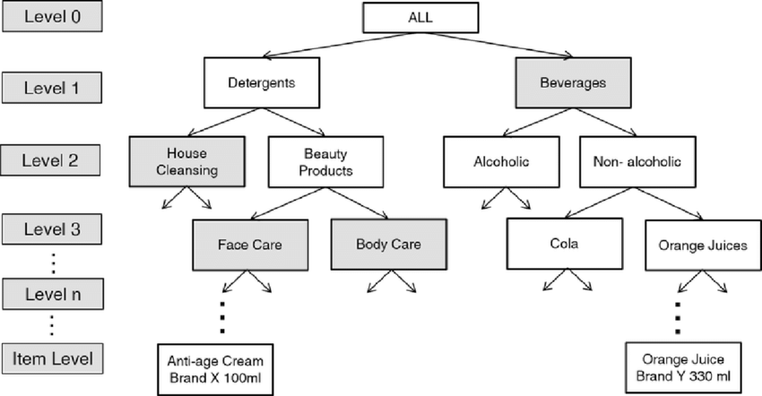
Category → a tree
Taxonomy distance = shortest path
Distance = path length up to a common ancestor and back down. A tree is a graph, so this is exactly the
shortest-path distance from Part III — and it is a metric on category nodes.
But distinct products in the same category have distance 0, so the representation, not the metric, is the limit.
Text → direction of a term vector
Cosine: similar wording, any length
cos(θ) = (a · b) / (‖a‖ ‖b‖) dcos= 1 − cos(θ)
Same meaning, different words → no shared terms → the vectors are orthogonal, cosine similarity 0.
Read it carefully
Only the direction of the term vectors matters, never their length — good for descriptions of different sizes.
Blind to synonyms: “car” and “automobile” share no terms, so cosine sees them as unrelated even though the docs mean the same thing. Dense embeddings (next lecture) fix this.
Also: distance 0 means same direction, not identical; and 1 − cos θ is not a true metric.
Price → Euclidean, but beware units
Standardize — then don’t over-trust it
Raw price dominates small-scale features, so standardize: z = (x − μ)/σ.
But equal scale ≠ equal relevance, and it does not remove outlier sensitivity — scaling is not a priority decision.
Reviews → sparse & cold-start
What about products with no history?
Most products have few reviews; brand-new ones have none (cold start).
The distance must degrade gracefully when a representation is missing or thin.
Reviews → a distribution over ratings
A distance over customer reviews
Each item → its rating distribution; the distance compares the two histograms.
Representation + distance
Encode each item by its rating distributionp = (p₁, …, p₅) — the fraction of reviews at each
star level. Then d(A, B) is a distance between the two histograms.
Average rating alone is too lossy — very different distributions can share a mean.
L1 / Euclidean on the histograms is simple, but treats every star as equally far apart.
Earth Mover’s (Wasserstein) respects order — 4★ vs 5★ is closer than 1★ vs 5★.
Two items have “similar reviews” when their distributions match — and few-review (cold-start) items need smoothing toward a prior.
Question
Your query is a running shoe. Ranked by price, the single closest product is a formal dress shoe. Is that a good recommendation — and what decides the answer?
Price crowns a dress shoe; text pulls in socks; only the right representation ranks the other
running shoe first. The distance is the model.
From objective to algorithm
Combine distances — weights are priorities
d(x,y) = wc·dcategory + wt·dtext + wp·dprice
Two cautions, linked
The terms must be on comparable scales before you add them — exactly the standardization point again.
The weights w encode priorities; they are the model’s hyperparameters. Standardization does not choose them for you —
you decide what should matter. Then rank the top-k neighbours and evaluate against real clicks/purchases.
Part V · Case study 2
Videos: which differences to ignore
Invariance, thresholds, and a system that scales.
YouTube: near-duplicates of an upload
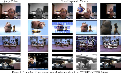
Equivalent for our task, different in the bytes
What should be ignored: re-encoding, modest colour changes, logos/overlays, small crops.
The job is the opposite of case 1 — choosing differences to discard.
Byte equality is the wrong tool
Exact ≠ near
The failure
Byte equality and cryptographic hashes (MD5, SHA) are designed so one changed pixel flips the whole digest.
They detect identical files, never perceptually similar ones.
We need a representation where small perceptual changes → small distance.
Construct the right representation
Perceptual hashing (pHash)
Each frame becomes a short fingerprint. We take the hash on faith — how it is computed is a black box here; all we need to trust is that similar frames give similar fingerprints.
The fingerprint survives re-encoding, small crops and overlays — so near-duplicate frames land on near-identical codes. We compare those codes next.
Compare → Hamming distance
Count the differing bits
a = 10110010 b = 10111010 → dHamming = 1
Back to Part III
Hamming distance is a proper metric on fingerprints — we verified all four axioms in Part III.
Yet distinct videos can share a fingerprint. A metric in the representation space does not guarantee the
originals are distinguishable — the same lesson as taxonomy-distance on products.
Make a decision, accept errors
Pick a threshold — trade off the two mistakes
Decision rule call it a near-duplicate when Hamming distance ≤ τ.
Threshold too tight → miss real duplicates (false negatives).
Threshold too loose → flag unrelated videos (false positives).
τ is chosen from data — exactly the kind of knob the task, not the metric, decides.
Generate a small candidate set cheaply (fingerprint buckets / LSH), then verify the few survivors with the
expensive comparison. Never materialise all n² distances.
The same shape powers web search, retrieval and question answering — a recurring pattern this year.
Synthesis
Change the distance, change the patterns
Why this one choice ripples through every task.
Back to the four tasks
Changing the distance changes the answer
Nearest neighbours change → classifications and recommendations change.
Neighbourhoods change → clusters and density estimates change.
What counts as “far” changes → detected anomalies change.
Case
Main lesson
Products
Choosing which differences matter
Videos
Choosing which differences to ignore
Take away · and a transfer exercise
Choosing a distance is choosing what you can see
The message
Task → representation → distance → decision. Metrics buy predictability and speed; but a valid metric and a
task-useful distance are two separate questions.
Choosing a distance is choosing which patterns an algorithm can see.
Transfer: for detecting duplicate news articles — what representation would you choose,
which changes should be ignored, and how would you evaluate the result?